9/28/2016 - Centripetal Acceleration vs Angular Frequency (Lab 8)

PURPOSE:
To determine the relationship between centripetal acceleration and angular speed.

THEORY:
We know that the net centripetal force of a rotating object is given by F = mrω². If we compare this equation to Newton's second law, F = ma, then it becomes apparent that if the net force equal mass times acceleration, then the net centripetal force must be equal to mass time centripetal acceleration. Therefore, a_cent = rω² = v²/r

APPARATUS:
The apparatus was assembled beforehand for this lab.

Wooden rotating disk with power supply and voltage regulator.

Setup:

1. Place the wireless accelerometer on the wooden disk.
2. Adjust the voltage on the power supply, turn the scooter motor on, and let the disk come to a constant speed.
3. Collect period and acceleration data for a variety of rotational speeds by varying the voltage.

EXPERIMENTAL PROCEDURE:

1. Use a photogate to measure the rotational period of the given mass.
2. Determine the mass of the object on the rotating disk.
3. Measure the radius of the object from the center of the disk.
4. Record the mean force exerted on the rotating mass.
5. Calculate the angular speed of rotating mass.
6. Repeat these steps 7-8 more times w/ varying ω and record them on a spreadsheet.

DATA/GRAPHS:

Recorded data

F vs. mω² 

F vs. rω²

F vs. ω²

Sample Calculation:
F = mrω²
F/(mr) = ω²
ω = [F/(mr)]^1/2
F = 2.35 N
m = 0.2 kg
r = 0.58 m
ω = 4.5 rad/s

ANALYSIS:
For this experiment, we made graphs of F vs. mω², F vs. rω², and F vs. ω². Ideally, each graph was supposed to have a slope of r, m, and mr respectively. If the slopes of the graphs match the variable that it is missing from the equation for centripetal force, then we have verified that the relationship between angular speed and centripetal acceleration is credible. The reason this method works is because it allows us to see how a change in a single variable can effect the others. For example, from F vs. rω², we can see that the slope of the linear fit of the graph is 0.2026, which is very close to the mass of the object on the wooden disk: 0.2 kg. The same hypothesis held true for the F vs. ω² graph, which yielded a slope value of  0.1249; a very close approximation of mr = 0.116. On the other hand, when we tested it with the graph of F vs. mω², we found that our prediction did not hold to be true. In fact, our data shows that the slope of the graph was 0.8249 when it  should have been closer to 0.58: the measured radius of the spinning mass.

CONCLUSION:
The data that we collected allowed us to analyze the relationship between centripetal acceleration and angular speed. More specifically, the graphs we created allowed us to illustrate how each of the variables we collected -- m,r, ω -- can effect this relationship. By comparing the slope of each graph to its corresponding "missing variable", we were able to successfully prove that centripetal acceleration did in fact depend on angular speed, among other factors. This mathematical relationship, however, was not entirely consistent with our data. Therefore, there must have been some uncertainty that was influencing our results. The most likely source of this discrepancy was human error. After comparing our group's data to another, we discovered that one of our data points for force varied by .05 N. Additionally, the other group used more data points in their graph for F vs. mω², which yielded a slope that was relatively more consistent with the radius of the mass around the disk. Another likely source of uncertainty in our calculations was our assumptions about the experiment. For example, when we began the experiment, we assumed that friction was negligible, when in reality there were many sources of friction because the wooden disk was in contact with several wheels while spinning.

GROUP MEMBERS: Xavier C., Billy J., Matthew I.

8/5/2016 - Work-Kinetic Energy Theorem Activity (Lab 11)

PURPOSE:
Prove that the work done when you stretch a spring through a measured distance is equal to the change in the kinetic energy of the spring.

THEORY:
If there are no external forces acting on the system, then ideally, the total work done to the system should be equal to the change in the kinetic energy of the system. For a non-constant force, such as a cart+spring on a ramp, the total work done can be calculated by finding the area under the force vs. distance graph. In a perfect world, the calculated area and the change in KE should be equal. In the world we live in, however, the accuracy of our calculations will depend on a variety of factors, such as the accuracy of our assumptions, the preciseness of our equipment, and the diligence of the people who perform the lab. In this experiment, we will explore how well our theoretical model of energy fits with reality.

APPARATUS:
We set up a ramp, cart, motion detector, force probe, and spring as shown in the diagram. One end of the spring is attached to a metal rod which is clamped to the table.

cart+spring system

EXPERIMENTAL PROCEDURE:
Part 1: Force vs. Distance

1. Calibrate the force sensor.
2. Set up the apparatus as shown.
3. Open the apt experiment file to display a force vs. distance diagram in Logger Pro.
4. Zero the force probe, verify the motion sensor is measuring toward the detector as the positive direction.
5. Sketch/Capture an image of the graph. Find the spring constant. Find the work done in stretching the spring using the integral function on Logger Pro.

Part 2: Kinetic Energy vs. Distance

1. Measure the mass of the cart.
2. Create a New Calculated Column for the KE of the system with respect to position.
3. Zero the force sensor and the motion detector at the desired starting position. 
4. Pull the cart back about 0.6 m, let it go, and begin graphing your KE data.
5. Compare the ΔK from points a,b to the area under the F vs. x graph through points a,b.

DATA/GRAPHS:
mass of cart = 0.756 kg
spring constant, k = 5.794 N/m

Force vs. Position Graph

KE vs. x and ∫ F(x)dx through points (a,b)

KE vs. x and ∫ F(x)dx through points (a,c)

KE vs. x and ∫ F(x)dx through points (a,d)

Δx - Work - Kinetic Energy - Data Chart

ANALYSIS:
We calculated the work done by the force of the spring by integrating the force function with respect to position. This method works because it is the equivalent of calculating the area under the force vs distance curve, which yields W = force*distance. After comparing it to the change in kinetic energy, our group found that the KE at the final position for a given range of values was approximately equal to the work done over the same set of values. For example, between the position values x = 0.51 m to x = 0.17 m, we found the work done between those points to be about 0.63 J, while the change in KE was about 0.83 J. In other words, we found that the change in KE was relatively close to the total work done on the system between those two points. On average, however, there was about a 24% difference between the two values, indicating a few sources of uncertainty in our experiment.

CONCLUSION:
Our data clearly illustrates that the change in the KE of our system did not entire coincide with the total work done over two points. However, while the reality of our calculations did not totally match up with their theoretical counterparts, this does not mean that the theory we tested is discredited. In reality, our data showcases how small changes in our methodology can influence irregularities in our calculations. In other words, there are several reasons why there was such a large disparity between the calculated work and the change in KE of the system. For instance, the lab equipment we used is not the best in the world. If we decided to buy and use more expensive and precise lab equipment, then we could have measured the mass, velocity, and force of the system with minimal error, which undoubtedly could have greatly increased the accuracy of our calculations.

GROUP MEMBERS: Xavier C., Billy J., Matthew I.

8/5/2016 - Conservation of Energy -- Mass-Spring System (Lab 12)

PURPOSE:
To determine whether or not energy is conserved in a vertically-oscillating mass-spring system, where the spring has a non-negligible mass.

THEORY:
In this experiment, we have a mass hanging from a uniform spring a certain distance above the ground. When the spring is a certain height above the ground, it has GPE. When it is released from this position, some of its GPE is converted into KE. If there are no other forces acting on the system, then the GPE will be converted into KE until the spring is in its equilibrium position. As the spring-mass system reaches its maximum displacement, all of its KE is converted into EPE. After the spring has stretched its maximum distance, the hanging mass will rise as its EPE is converted back into KE. As the spring-mass system oscillates, this energy cycle continues until external forces such as friction retard the spring to a standstill. If energy is conserved, then the total energy of the system will be constant. However, in order to take the mass of the spring into account for our energy calculations, we must derive new formulas for GPE and KE using calculus.

APPARATUS:
We hung a 200 g mass on a hanger for a total mass of 250 g. The bottom end of the spring is holding the mass, while the top side is hanging from a horizontal metal rod, which is fixed to another metal rod that is clamped to the lab table.

We also attached a force sensor to the horizontal metal rod, such that the spring could hang from it with the hanging mass attached. Additionally, we placed a motion sensor beneath the spring-mass system. Lastly, we taped a flashcard to the bottom of the hanging mass to make it easier for the motion sensor to detect.

Apparatus: Part 2

EXPERIMENTAL PROCEDURE:
Part 1: Determine the Spring Constant

1. Calibrate the force sensor.
2. Set up Apparatus: Part 2, as shown. Note: Remember to zero the force sensor when spring is attached.
3. Calibrate motion sensor.
4. Collect Force vs. Time data and Stretch vs. Time data. 
5. Plot a Force vs. Stretch graph to obtain an equation for the force of the spring. (F = kx + F0)
6. Holding the mass+spring system from its equilibrium position, use the motion detector to determine its position relative to the "ground." (i.e. from the front of the motion sensor).
7. Make a new Calculated Column called "Stretch." This equation will be based on the motion sensor reading.

Part 2:

1. Hang 200 g on the mass hanger for a total mass of 250 grams.
2. Pull the spring down about  10 cm and let it go. 
3. Record position and velocity graphs and sketch them in your lab module.
4. Make prediction sketches of KE vs. time, GPE vs. time, and EPE vs. time.
   
   

   

   Energy Prediction Sketches

5. Now, set up Logger Pro to calculate the various energies in New Calculated Columns.
6. Use Logger Pro to produce plots of KE vs. y, KE vs. v, GPE vs. y, GPE vs. v, EPE vs. y, EPE vs. v.

Here are the equations we used for various energies, *Note: We derived them in class using calculus:

KE = (1/2)[mhanging + (1/3)mspring]v^2

GPE = [mhanging + (1/2)mspring]gy

Elastic PE = (1/2)k(stretch)^2

DATA/GRAPHS:
Part 1:
mspring = 86.0 g
mhanging = 350 g
k = 5.794

Part 2:

GPE vs. t - KE vs. t - EPE vs. t 

KE vs. y

KE vs. v

GPE vs. y - EPE vs. y

GPE vs. v - EPE vs. v

GPE vs y -EPE vs. y - Energy Sum (for each)

GPE vs. v - EPE vs. v - Energy Sum (for each)

ANALYSIS:
After analyzing my energy data and comparing it to my predictions, it is apparent that I made a few incorrect assumptions. For example, when I created my sketches, I predicted that GPE would increase at the same rate EPE would decrease and vice versa. I made this prediction because GPE should be at its lowest when EPE is at its highest. This, however, was not the case at all according to our data. In fact, my data illustrates that my prediction is the antithesis of what happens because both the GPE and EPE oscillate together at very similar rates. Another error I made in my prediction was that I took the EPE of the system to be positive when in reality it is negative because it acts in the opposite direction of the spring force (which is in the positive direction for this experiment). In order to verify that our data was consistent with our physical model, we also analyzed our energy vs y and energy vs. v graphs. Our KE vs. v,y graphs made sense because they they were both consistent with the increase in the speed of the system. Our GPE, EPE vs. y graphs were logically sound because they both increased and decreased respectively with respect to the height relative to the motion sensor. Moreover, our GPE, EPE vs. v graphs had warranted values because they are both reach their max when the KE decreases to zero.

CONCLUSION:
Overall, our group was able to successfully demonstrate that the energy of the mass+spring system was conserved because our data showed that the total energy of the system remained nearly constant throughout. However, the lines that Logger Pro displayed were not as straight as we hoped they would be. Therefore, there could have been a few sources of uncertainty in our experiment that we did not account for. One of the many possible sources of error we encountered were external forces acting on the system. This includes, but is not limited to: air resistance caused by the flashcard, damping caused by dissipated heat due to friction, and permanent spring deformation. Another possible source of uncertainty was through human error. For instance, if we inaccurately recorded length measurements, then the preciseness of our initial data would be negatively affected, thereby decreasing the accuracy of our energy calculations.

GROUP MEMBERS: Xavier C., Billy J., Matthew I.

8/10/2016 - Magnetic Potential Energy (Lab 13)

PURPOSE:
To verify that conservation of energy applies to a system with magnetic potential energy (MPE).

THEORY:
Consider a cart with a strong magnet sliding along a level air track with another magnet of the same polarity fixed at the other end. As the cart moves along the track, it will have some KE. However, as the cart approached the end of the track, its KE will reduce to zero and all of the energy will be stored in the magnetic field as MPE, then it rebounds back. Since the MPE is not constant, we will use the relationship U(r) = -∫ [r,∞] F(r)dr to relate our MPE to the separation distance, r.

APPARATUS:
We used a glider on a frictionless track. The glider has a strong magnet attached to one end and at the end of the track there is another magnet with the same polarity. On top of the glider, there is a thin aluminum plate that is used to facilitate the collection of position data with a motion sensor, which is located at the same end of the track as the magnet.

EXPERIMENTAL PROCEDURE:
Part 1: Force Equation

1. Prepare apparatus as shown.
2. Weigh cart+reflector.
3. Connect vacuum hose to air track.
4. Calibrate and connect motion detector with Lab/LoggerPro.
5. Tilt the air track at various angles in order to create a relationship between the magnetic force, F and separation distance, r.
6. For a given angle θ, use calipers to record the separation distance, r between the two magnets.
7. Plot a graph of F vs. r. We assume that their relationship is a power type equation of the form: F = Arⁿ. 
8. Get the A and n values from the curve fit of your F vs. r graph. 
9. Integrate the force function to get your equation for the MPE. 

Part 2: Verification

1. With the air turned off, place the cart+reflector reasonably close to the fixed magnet at the end of the track. Run the motion detector. Determine the relationship between the the distance the motion detector reads and the separation distance between the two magnets. Assuming that the distance between the the reflector and magnet of the cart is negligible, the distance r = P - k.
2. Use the motion detector and LoggerPro to measure the speed and the separation between the two magnets.
3. Start the cart at the far end of the track, turn on the air track, and give the cart a gentle push.
4. Record data necessary to to verify that energy is conserved.
5. Create a graph of KE, MPE, and total energy as a function of time.

DATA/GRAPHS:

Data from Part 1

Sample Calculation of Fmag (Part 1)

Curve Fit of Force vs. Time

Derivation of Magnetic Potential Energy Function

KE-MPE-TE vs. Time Graph

ANALYSIS:
In order to verify that energy was conserved for this experiment, all of the KE of the cart must be transferred into MPE when the cart is just about to rebound. As the cart travels down the air track at a constant speed, the kinetic energy remains constant. Moreover, as the cart approaches its minimum distance between the two magnets, the KE exponentially decreases as the MPE increases at an identical rate. Since it appears that the KE reaches zero at the same time the MPE reaches its maximum, it is safe to conclude that energy was conserved for this experiment. Another way we know that energy was conserved is if the total energy (TE) of the system remains constant. If the TE of the system decreased over time, then this would imply that a net external force acted on the system, causing some of the initial KE to be lost in the process. However, since our line for the total system energy stayed relatively constant throughout, it is safe for us to conclude that energy is conserved.

CONCLUSION:
Our group was able to successfully create an equation for the MPE of the system that showcased the energy of the system was relatively conserved. However, there is some uncertainty in our calculations because our line for the total energy of the system is not as straight as we had hoped. This tells us that there was most likely a net external force acting on the system from sources we did not take into account. For example, if the track was unleveled or was not uniformly frictionless, then the speed of the cart could have been hindered by friction or gravity. Furthermore, the inaccuracies in our energy calculations could have also resulted from the imprecise measurement of the separation distance, r, the distance between the motion detector and the magnet, the angle of incline, or even the mass of the  cart+reflector. If we used more precise equipment, a perfectly level and frictionless surface, and minimal human error, then we could expect to see a more straight TE line, indicating that the energy of our system was indeed fully conserved.

GROUP MEMBERS: Xavier C., Billy J., Matthew I.

8/12/2016 - Ballistic Pendulum Lab

PURPOSE:

Determine the firing speed of a ball form a spring-loaded gun.

THEORY:
The ball, mass m, undergoes an inelastic collision with a nylon block, mass M. We assume that the collision happens so quickly that the strings stay vertical throughout the entire collision. This allows us to use conservation of momentum to write an equation for the speed of the system after the collision.

After the collision, the block+ball system rises, losing KE and gaining GPE until it reaches its maximum height. We can use the conservation of energy to write an expression that relates the maximum height to the initial speed of the block.

APPARATUS:
In this lab, the apparatus comes pre-assembled. A spring-loaded gun fires a ball into a nylon block, which is supported by four strings. The ball is absorbed into the block, and the ball and block rise together through some angle, which is measured by the angle indicator.

EXPERIMENTAL PROCEDURE:
Part 1: Initial Velocity

1. Measure/record the mass of the ball and block.
2. Level the block and apparatus.
3. Pull back and lock the spring into one of the notches. (Keep this notch consistent)
4. Fire the ball and record the max angle it travels through.
5. Repeat this 4-5 times to get an average.
6. Calculate the firing speed of the ball.

Part 2: Verification

1. Move nylon block away. 
2. Prepare the apparatus to launch the ball off the table.
3. Place a piece of carbon paper over another piece of paper close to where you expect the ball to land.
4. Determine the actual launch speed of the ball.

DATA:
Part 1:

Part 2:

height of barrel from floor: 0.97 meter

distance traveled by ball: 2.52 meters

ANALYSIS:
Initial Velocity:

Energy and Momentum Approach

Propagated Uncertainty Calculations

Verification:

Kinematics Approach

Propagated Uncertainty Calculations 2

ANALYSIS:

The ballistic pendulum lab is a classic example of an inelastic collision, i.e. a collision between two objects that stick to one another afterwards. Since this collision is inelastic, the momentum of the system is conserved before and after the collision. Energy, on the other hand, is not conserved before and after because there is an inherent loss of KE in the system when the two colliding masses merge with one another. However, since there is presumably no net external force acting on the system after the collision, energy is conserved after the collision, as the bullet+ball system rises with KE and reaches its maximum height with nothing but GPE. After calculating the initial speed of the bullet with our energy and momentum equations, we yielded 6.02 +/- 0.15 m/s. After calculating the initial speed using kinematics, however, we yielded 5.64 +/- 0.00364 m/s. These results have an unacceptable margin between each other because they are not within even the respective upper and lower ends of our propagated uncertainty calculations.

CONCLUSION:

Our results for this experiment were unsatisfactory. After calculating the initial speed of the bullet with our energy and momentum equations, we yielded answers for the initial velocity of the bullet that had an unacceptable margin between each other. There are several factors that could have contributed to this uncertainty. If, for instance, the nylon block remained unbalanced, then our calculations for initial velocity would be inherently flawed because momentum would not have been conserved. Another source of uncertainty is in human error. In our group's case, we had up to twelve different people trying to work together while a handful of people made their own measurements. This chaos increased our chances of miscommunication, potentially leading to imprecise measurements for the whole group. 

GROUP MEMBERS: Xavier C., Billy J., Matthew I.

10/19/2016 - Collisions in Two Dimensions (Lab 15)

PURPOSE:
To look at a 2-D collision and determine if momentum and kinetic energy are conserved.

THEORY:
In collisions where there are no external forces acting on the system, both momentum and kinetic energy are conserved. In this experiment, we want to see if these principles apply to a collision between two balls on a frictionless surface. To test this, we calculate the kinetic energy (KE = .5mv^2) and momentum (p = mv) before and after the collision. If the before and after values are nearly identical for the respective quantity of motion, then the collision is elastic.

APPARATUS:
We used a leveled glass table as our frictionless surface. For our collision objects, we used a glass marble and a steel ball. To capture the collision in slow-motion, we used a ring stand to suspend a smartphone with the capability to record at 120-240 fps.

EXPERIMENTAL PROCEDURE:

1. Gather appropriate materials.
2. Set up apparatus as shown.
3. Make sure glass table is leveled.
4. Measure length of glass table.
5. Place marble in the center of the table.
6. Set up smartphone to record in slow-motion.
7. Mount phone onto ring stand.
8. Record the two following collisions separately:
9. Aim and roll a steel ball towards the marble.
10. Aim and roll another marble towards the marble.
11. Transfer these video files to LoggerPro.
12. Input your table length measurement to calibrate your video tracer.
13. Adjust the click rate to 4-8 frames.
14. Trace the position of the each ball separately for each collision.
15. Get the velocities of each ball before and after each collision.
16. For each collision data set, create two calculated columns that show the momentum in both the x and y axes.
17. Finally, create graphs for the position and velocity of the center of mass in both the x and y axes.

DATA/GRAPHS:
mass of marble (middle): 19.6 g
mass of second marble: 19.8 g
mass of steel ball: 66.9 g
Length of glass table: 0.625 m

Marble-Marble Collision

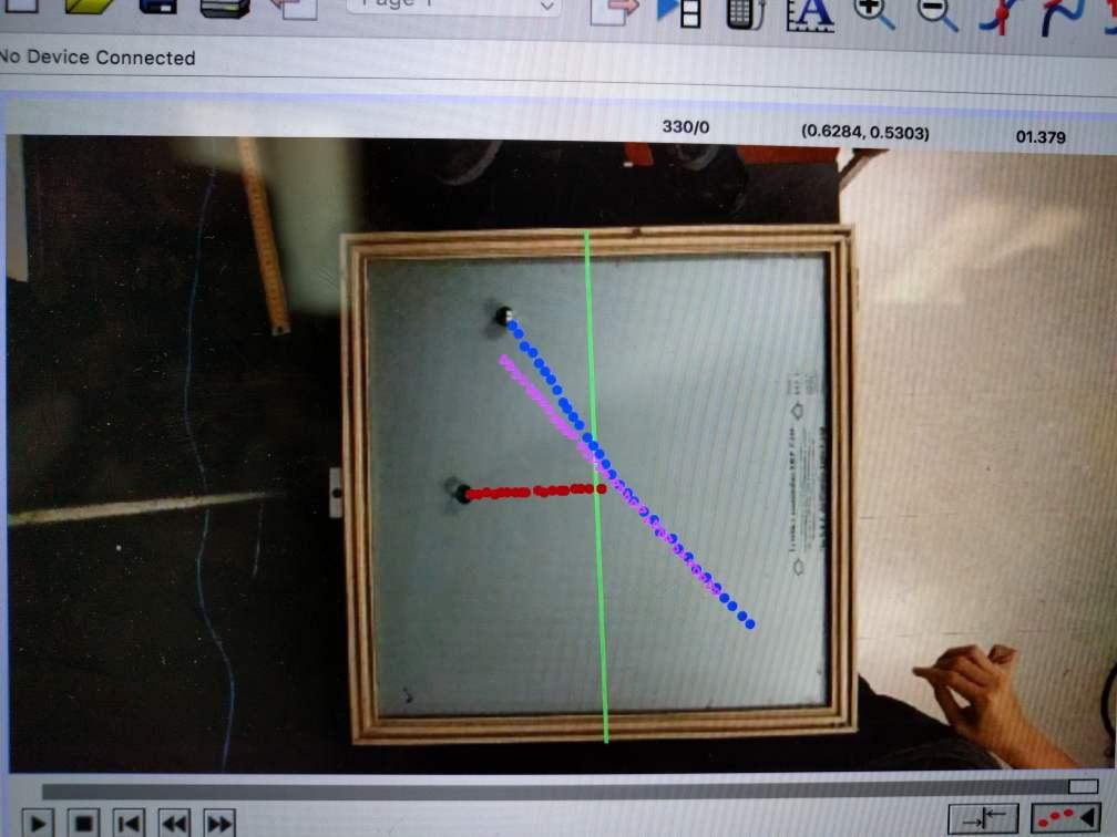
Marble-Marble Position Graph

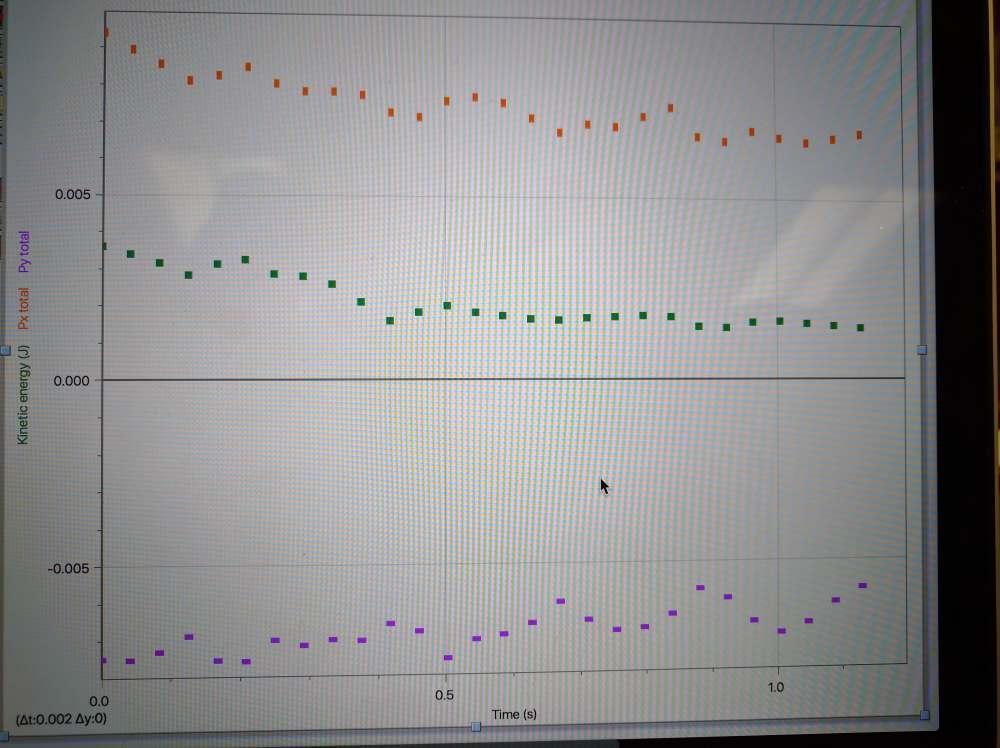
KE-Px-Py for Marble-Marble Collision

CM Position for Marble-Marble Collision

CM Velocity for Marble-Marble Collision

Steel Ball-Marble Collision

Steel Ball-Marble Position Graph

KE-Px-Py for Steel Ball-Marble Collision

CM Position for Steel Ball-Marble Collision

CM Velocity for Steel Ball-Marble Collision

ANALYSIS:
By simulating a collision between two balls with different masses, we were able to analyze their behavior to determine whether or not momentum and energy were conserved. However, instead of doing the calculations by hand, our group decided to derive equations that could be inputted into a calculated column for both momentum (x and y) and kinetic energy for each collision respectively.

KE-Px-Py Equations for LoggerPro

If momentum is conserved, then the the momentum in the x-axis should be equal but opposite to the momentum in the y-axis. In other words, if our graphs for Px vs. t and Py vs. t are nearly identical but opposite in value, then momentum is conserved. If kinetic energy is conserved, then we should expect to see that the KE vs. time graph should be nearly constant.

After analyzing our graphs, it becomes apparent that the momentum for both collisions appear to be conserved. However, it is less apparent to see that the kinetic energy is conserved. The collision between the two marbles yielded a relatively straight line, but the collision between the steel ball and the marble had an erratic line, indicating that the kinetic energy throughout the collision varied greatly.

CONCLUSION:
Our results for this experiment were somewhat bittersweet. On the one hand, we successfully demonstrated that the momentum of both collisions were conserved. On the other hand, we had difficulty verifying the same was true for the kinetic energy of both systems. We assumed that there were no external forces acting on the system, although there is bound to be some inherent uncertainty to this statement. For example, if the glass surface we used was unclean, it could have gathered residue, which could have inadvertently hindered the speed of the ball. Another possible source of uncertainty is human error. The motion tracking software on LoggerPro utilizes human input, which can lead to the imprecise collection of data for the position, velocity, and to that end, all of our momentum and KE computations as well.

GROUP MEMBERS: Xavier C., Billy J., Matthew I.

10/3/16: Centripetal Force with Motor (Lab 9)

PURPOSE:
To create an expression that models the relationship between angular velocity, ω, and angle, θ, for a mass revolving around a central shaft.

INTRODUCTION:
As the motor spins at a higher angular speed ω, the mass attached to the central rod revolves at a larger radius and the angle θ increases. From this experiment, we can quantitatively define a relationship between angular speed and angle measure. The goal of this lab, therefore, is to derive an expression that defines ω in terms of θ. After this is done, we will test the accuracy of our model by comparing it to another method for calculating angular speed ω in terms of time, t.

APPARATUS:
Note: the apparatus was pre-assembled for this particular lab.

The real apparatus (top) and a diagram (bottom):

• An electric motor mounted on a surveying tripod 

• A long shaft going vertically up from the motor.

• A horizontal rod mounted on the vertical rod. 

• A long string tied to the end of the horizontal rod. 

• A rubber stopper at the end of the string. 

• A ring stand with a horizontal piece of paper or tape sticking out.

We utilized the apparatus to derive some key variables before proceeding with the experiment. For example, our group:

• Derived θ by looking at the right triangle -- from the diagram above -- with hypotenuse L and height H-h. Equation: θ = arccos((H-h)/L)
• Derived ω from timing the duration for the mass to make a number of revolutions around the shaft. Equation: ω = 20π/Δt (20π because we did ten rotations)
• Derived h by putting a horizontal piece of paper on a ring stand and slowly raising the piece of paper until the stopper just grazed the top of it as it passed by. Equation: None, just a ruler.

PROCEDURE:

1) Use a free body diagram (FBD) to create centripetal force equations of the system. Use these equations to create a mathematical model for ω in terms of θ. Here is our derivation of ω:

2) Use the apparatus to gather a sufficient amount of data to test your model. More specifically, you must collect values of h at a variety of values for ω. The professor adjusted ω by increasing the voltage to the motor driving the system.

3) Create an Excel Spreadsheet with the following variables: t, h, H-h, θ, ω (t), ω (h).

4) Create a graph of angular speed with respect to time t vs. angular speed with respect to angle θ.

DATA/GRAPHS:
Uncertainty in  r, L, and H: +/- 0.1 cm
Uncertainty in t: +/- 0.25 s (due to reaction time)
Uncertainty in h, H-h: +/- 0.1 cm

ω(t) = angular speed with respect to time.
ω(h) = angular speed with respect to θ.

***In chart "r" = "R" on the apparatus diagram.

Data Table with Relevant Variables and Constants

ANALYSIS: 

There are two forces acting on the stopper as it is spinning: tension and gravity. The horizontal component of tension is providing a net centripetal force on the rubber stopper, helping it accelerate towards the center and rotate at a constant speed. Since the stopper is not moving in the y-direction, Newton's first law dictates that the net force must be equal to zero. Therefore, we now know that the vertical component of the tension force is equal in magnitude but opposite in direction to the weight of the rubber stopper. Using these principles, we formulated our force equations, manipulated them, and solved for angular speed ω. The slope of the previous graph, therefore, represents the accuracy of our derived value of ω with respect to θ. The slope is in the form: 1 + uncertainty in ω(θ), (where ω(θ) is angular speed with respect to theta). Additionally, R² represents the correlation value of our graph. In other words, it quantifies how close our linear fit of the data came to matching all of our data points. According to our graph, we accumulated an uncertainty of about 4.82%.

CONCLUSION:

Overall, our calculation of angular speed with respect to an angle was very accurate. This is because our expression for ω(θ) calculated a value for angular speed that was within 5% of the angular speed we calculated with respect to time. While some 4A students would be satisfied with this minute margin of error, I for one find it much more satisfying to explore the ways in which our group could have mitigated a multitude of these myriad mistakes. The first step in minimizing this uncertainty is identifying the root causes. One of the main causes of uncertainty in our lab was human error. For example, it is possible that our group mate inaccurately measured the period of rotation due to our inherent lag known as "reaction time." Moreover, it is also possible that we could have inaccurately measured distances on the apparatus by a small margin as well. This is because the tick marks on the meter sticks can be difficult to distinguish at times and different perspectives can lead to inconsistencies over the most precise measurement. Another source of error in our lab were variables we omitted from our calculations. For instance, our class decided that air resistance due to drag was negligible. Thusly, we did not take drag force into consideration when creating our FBD and force equations. Another source of uncertainty in our calculations arose from the reverberation of the ruler atop the central shaft. As the motor spun the central shaft, the ruler would slightly oscillate, causing the radius of rotation to change as well. For the simplicity of the lab, however, our class decided that this effect was negligible as well and we treated the radius r as a constant for a given angular speed ω. In an ideal world, our group would redo this lab with top notch equipment and extreme attention to detail, but in recognition of the technical limitations and time constraints of a 4A class, our group accepts that our current experimental results will suffice. 

GROUP MEMBERS: Matthew I., Xavier L., Billy J.